Simulation and Control of iRobot Navigation
Project Snapshot
- Project Title: Simulation and Control of iRobot Navigation
- Type: Course Project - MECH 563 Industrial Robotics (DOCX)
- Project Report: View Report (PDF)
- Concepts:
- Localization
- Mapping
- Path Finding
- Robot Simulation
- Sensor Fusion
- Robot Kinematics and Dynamics
- Duration: Fall 2023
- Skills Developed:
- Robotics Simulation: Gazebo, ROS2
- Computer Vision: OpenCV, Stereo Camera Calibration
- Programming: Python, pycreate2 library
- Mapping, Localization and Path Finding: OctoMap, AMCL, Nav2
- Others: Docker, RViz
Project Overview
Abstract
For our project, we originally set out to accomplish two goals. Our first goal was to find a way to navigate an iRobot to any reachable pose within a 2D grid environment, while our second goal was to program the iRobot to reach a pose while avoiding collisions with objects within its actual environment. While our first goal was accomplished almost instantly by our discovery of the pycreate2 library package, we did not achieve our second goal of setting up a semi-autonomously navigating iRobot due to issues with stereo camera calibration, and the resulting complication which arises when trying to convert a disparity map into a point cloud. Nevertheless, this report will go through the work we’ve been able to do on stereo camera calibration, communicating sensor and actuator signal between the iRobot and a processor, and simulating the iRobot in a 3D environment using Gazebo and ROS2.
Figure 1: Demonstration of mapping of environment using Gazebo and Rviz2.
Introduction and Background
Features of the iRobot
The iRobot Create 2 used for this project is a programmable robot based on the Roomba vacuum cleaner (iRobot, 2024). It consists of a circular body with two driving wheels on the bottom. The other critical components of the iRobot are its sensors, primarily its bumper sensor which detects collisions from obstacles, and its cliff sensors to avoid any sudden drops. Furthermore, we planned on mounting a stereo camera on top of the iRobot which would allow the iRobot to map its surroundings and avoid colliding with obstacles. Lastly, the iRobot has an internal processor which allows us to send control signals and receive sensor input through the iRobot Create 2 API.
Methodology
1. Control Loop
Our original strategy for controlling the iRobot can be found in the figure below. One would begin by picking a point using Gazebo for the iRobot to travel to. Then NAV2 would subsequently lay out an approximately optimal trajectory which would follow this path. For every iteration of the outer-loop we calculate a new trajectory, whereas for every iteration of the inner-loop we apply PD control to make our iRobot travel a fixed trajectory. We exit the control loop once the iRobot’s current position (\(x_0, y_0\)) is sufficiently close to the destination (\(x_d, y_d\)). The iRobot keeps track of its current position using SLAM (Simultaneous Localization and Mapping).

Figure 2: iRobot control loop.
2. Kinematics and Dynamics
The iRobot utilizes two motors that drive individual wheels which allows for movement in forward and backward directions in addition to rotation of the robot. A kinematic diagram of the iRobot can be found below. We have that \(v_R\) and \(v_L\) correspond to the tangential velocity of the right and left wheel while \(\omega\) is the angular velocity of the iRobot’s body with respect to the global coordinate frame, about the center of mass of the iRobot. Furthermore, \(D\) is the distance between the two wheels and \(r\) is the radius of the individual wheels.
The robot’s equations of motion are controlled by the angular velocity of each wheel. The relationship between translational and tangential velocities are given by:
\(v_R = r \cdot \omega_R\)
\(v_L = r \cdot \omega_L\)
\(v = \dfrac{v_L + v_R}{2}\)
\(\omega = \dfrac{v_L - v_R}{D}\)
Let \(x\), \(y\), and \(\theta\) be the coordinates and orientation of the iRobot in the global coordinate frame. Then we have:
\(\dot{\theta}(t) = \omega(t)\)
\(\dot{x}(t) = v(t) \cdot \cos(\theta(t))\)
\(\dot{y}(t) = v(t) \cdot \sin(\theta(t))\)
It's important to note that we're assuming the environment in which the iRobot operates is entirely flat and provides constant friction. Further, we assume that the iRobot's wheels do not have a significant moment of inertia.
Let \(F_L\) and \(F_R\) be the tangential forces applied to the left and right wheels from the wheels acting on the floor due to a change in velocity (acceleration or braking). We can further derive the robot's translational acceleration to be equal to \(a(t) = \dfrac{F_L + F_R}{m}\), and the angular acceleration to be equal to \(\epsilon(t) = \dfrac{D}{2I}(F_L - F_R)\) where \(I\) is the moment of inertia of the iRobot.
Finally, using Lagrangian mechanics, we can derive the equations of motion for the iRobot:
\(u_L = I \cdot \epsilon_L(t) + F_L \cdot \omega_L(t) + F_L \cdot r\)
\(u_R = I \cdot \epsilon_R(t) + F_R \cdot \omega_R(t) + F_R \cdot r\)
Where \(\epsilon_L\) and \(\epsilon_R\) are the angular accelerations of the left and right wheels respectively. We can now define a linear state-space dynamics model with a state vector defined as \(x = [v, \omega, \omega_L, \omega_R]^T\), with its time derivative being \(\dot{x} = [a, \epsilon, \epsilon_L, \epsilon_R]^T\). Lastly, define the control input to be \(u = [F_L, F_R, u_L, u_R]^T\). We can now rewrite our dynamics as:
\(\dot{x} = A x + B u\)
Where \(A\) and \(B\) are matrices representing the system dynamics and control input coefficients respectively. Originally, we planned to apply a control algorithm on top of the iRobot’s dynamics model in order to get it to follow a trajectory planned by NAV2. Unfortunately, we never reached this part due to time constraints.
3. Camera and Image Processing
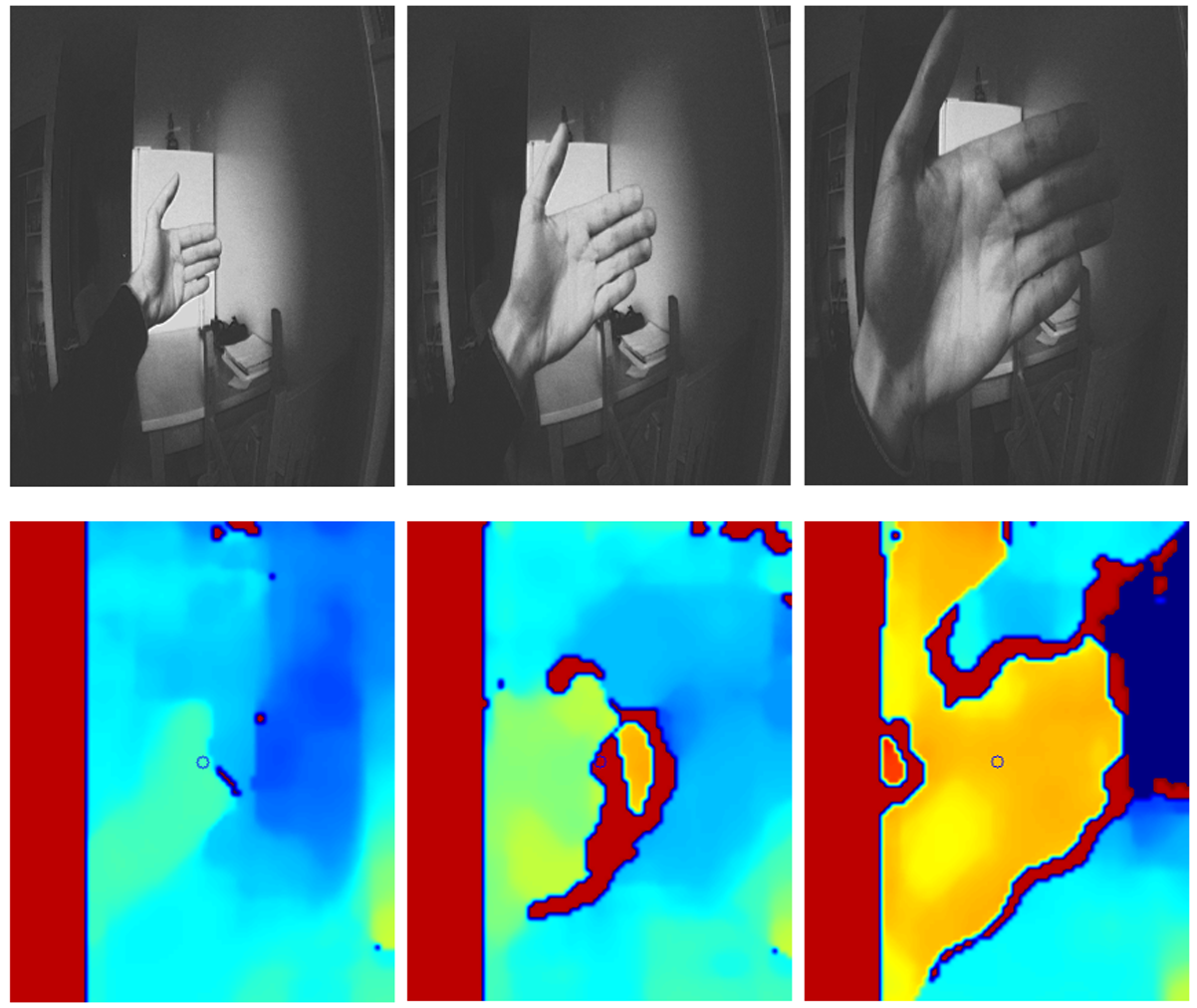
Figure 3: The disparity map after camera rectification and preprocessing for object detection.
In order to obtain accurate point cloud information and a cleaner disparity map, it was necessary for us to calibrate the stereo camera. The procedure for doing so involves taking dozens of pictures of a checkerboard at varying poses and distances from the camera, and using the two sets of pictures in order to estimate several parameter matrices. In order to accomplish this, we used the Python StereoVision library which is mostly based off of OpenCV. For stereo camera calibration in particular, the StereoVision library utilizes OpenCV methods like cv2.stereoRectify() and cv2.stereoCalibrate(). One of the matrices computed through rectification is the 4x4 perspective transformation matrix \(Q\), which is crucial for obtaining a point cloud downstream.
We used the StereoSGBM algorithm to compute a disparity map using two grayscale images given by the stereo camera. StereoSGBM works by matching uniformly-sized blocks of pixels between two cameras, and computes the disparity of a given block by measuring the difference in location of that block within the two corresponding image arrays. In order to get this to work, we had to do a fair amount of hyperparameter tuning in order to get a smooth map which presents closer objects as having higher disparity values.
4. Simulation of iRobot
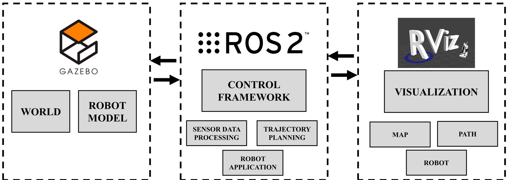
Figure 4: Simulation framework for iRobot.
In this section, we describe the methodology used for simulating the iRobot using the Gazebo simulation environment. Gazebo allows for the creation of complex three-dimensional scenarios on a computer, featuring robots, obstacles, and various other entities. It incorporates a physics engine to simulate real-world physical phenomena such as lighting, gravity, and inertia. This capability enables time-efficient evaluation and testing of robotic behaviors in challenging or hazardous conditions without risking damage to the physical robot.
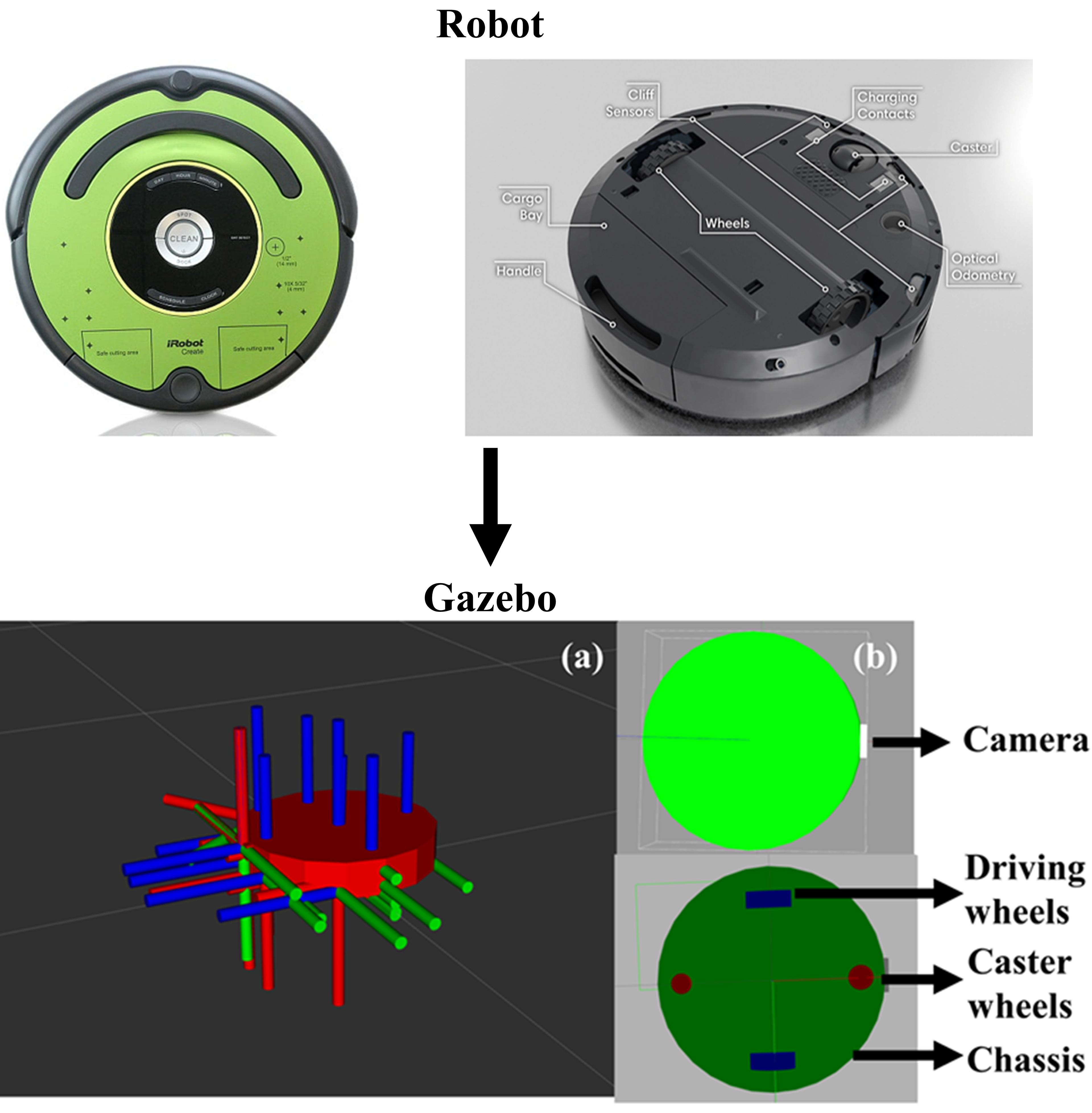
Figure 5: Modelling of iRobot using URDF.
We created a URDF (Unified Robot Description Format) file comprising links and joints, constructing a model of an iRobot. The chassis is represented by a cylinder with appropriate dimensions. Two driving wheels and two caster wheels are then attached to the chassis, with distances and radii approximating those of the actual iRobot. Additionally, a camera is defined as a simple cuboid affixed to the front of the chassis. The weights of each component are estimated and integrated into the model.
Gazebo plugins were used for the sensors: (i) libgazebo_ros_diff_drive for the differential drive, and (ii) libgazebo_ros_camera for the stereo camera, which captures the depth image. The differential drive plugin receives cmd_vel commands, allowing the robot to navigate within the virtual environment. The camera plugin publishes both raw images and depth images in the PointCloud2 format.
5. Mapping using OctoMap
OctoMap is a 3D mapping framework for robotic navigation and exploration. It models occupied and free spaces, with unknown areas implicitly encoded. The map can be continuously updated, incorporating new sensor data to adapt to changes in the environment and allowing for contributions from multiple robots. In this project, we use the depth camera as our sensor input in the format of PointCloud2 and create 3D voxels based on the height of the points in the cloud.
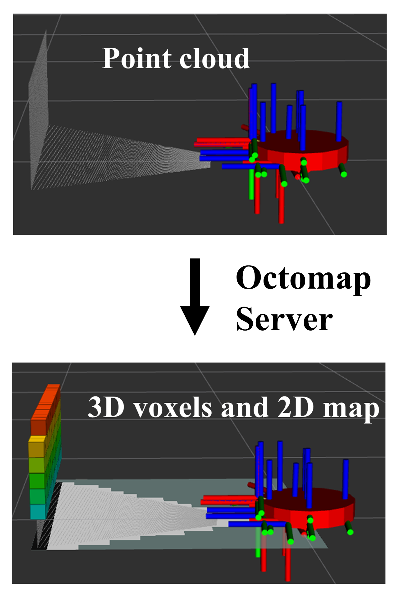
Figure 6: Mapping using Octomap.
6. Localization using AMCL
Adaptive Monte Carlo Localization (AMCL) is a probabilistic localization method widely used in robotics, particularly in ROS. AMCL works by integrating point cloud sensor data with an existing map of the environment, using a particle filter approach to estimate the robot's position and orientation. The algorithm continuously updates its estimates by sampling particles and weighting them based on their consistency with the observed sensor data. This process allows AMCL to provide accurate and robust localization even in dynamic environments.
7. Navigation
Once localized, the navigation stack publishes global and local cost maps. The global cost map is generated using the pre-existing static map, with parameters such as robot radius and buffer layers adjusted to suit our needs. The navigation stack utilizes this cost map to compute an optimal path using Dijkstra's algorithm. Additionally, a local cost map is generated, which acts as a controller, guiding the robot to follow the global path.
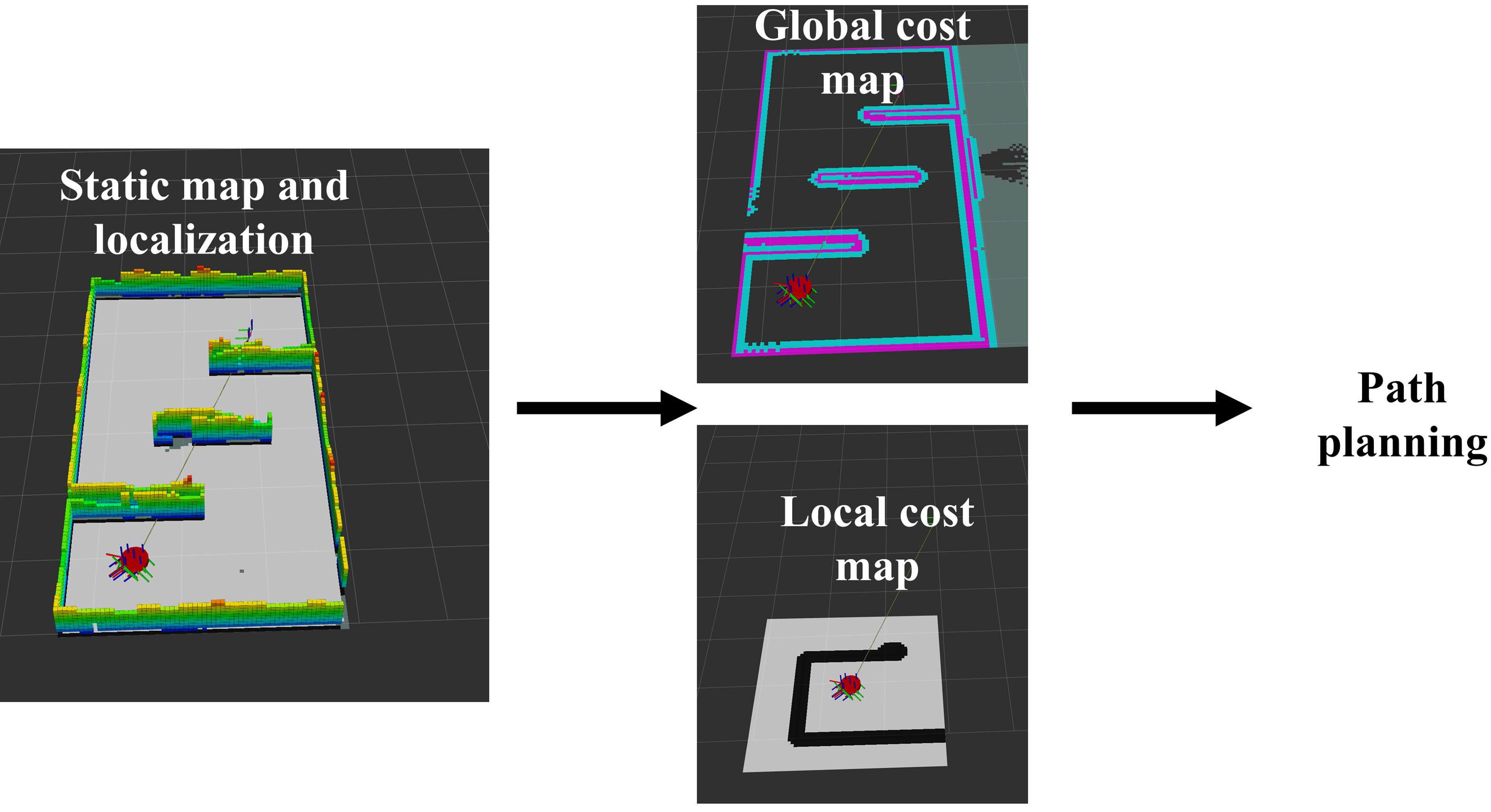
Figure 7: iRobot navigation stack.
Achievements
Throughout the project, we accomplished the following:
- Dockerized Workspace: We created a Dockerized workspace and posted it on GitHub for public access. This workspace can be run on any system, with setup instructions provided in the README file.
- iRobot URDF Model: We developed an iRobot model in URDF, incorporating the necessary links, joints, and sensors through Gazebo plugins.
- Custom Test World: We designed a custom test world to run our simulations and implement our algorithms.
- Mapping with OctoMap: We coded custom launch files for mapping the environment using OctoMap, utilizing point cloud data to represent the environment.
- Navigation Stack Parameters: We tuned and modified the parameters of the navigation stack to suit our robot, replacing conventional LaserScan data with point cloud data from the camera.
- Navigation Launch File: We developed a launch file for the navigation of the iRobot within a static map, enabling autonomous movement along pre-defined paths.
- Controlling the iRobot: We successfully used the
pycreate2package for controlling the iRobot, including testing its functionality and sensors. - Stereo Camera: We managed to significantly improve the disparity map quality for the stereo camera over its initial performance.
- Model Dynamics: We found a kinematics model which accurately models the iRobot and which could be used for control.
Conclusions
Summary of Findings:
- We successfully navigated an iRobot to any reachable pose within a 2D grid environment using the pycreate2 library package.
- Although we faced challenges with stereo camera calibration and converting disparity maps into point clouds, we made significant progress in these areas.
- We developed a comprehensive simulation environment using Gazebo and ROS2, which includes mapping, localization, and navigation capabilities.
Future Work:
- Complete the implementation of collision avoidance by improving the stereo camera calibration and point cloud generation.
- Rather than relying on the stereo camera, we could use a monocular camera, such as a smartphone camera, to implement ORB-SLAM (Oriented FAST and Rotated BRIEF Simultaneous Localization and Mapping).
Final Remarks
This project demonstrates the integration of robotics simulation, control, and computer vision to navigate an iRobot in a simulated environment. Despite challenges, we established a solid foundation for future work in autonomous navigation and obstacle avoidance. The tools and methodologies developed here can be extended to more complex scenarios and real-world applications.